r.futures.simulation - GRASS manual

NAME

r.futures.simulation - Simulates landuse change using FUTure Urban-Regional Environment Simulation (FUTURES).
Module uses Patch-Growing Algorithm (PGA) to simulate urban-rural landscape structure development.

KEYWORDS

raster, patch growing, urban, landscape, modeling

SYNOPSIS

r.futures.simulation

r.futures.simulation --help

r.futures.simulation [-s] developed=name subregions=name [subregions_potential=name] predictors=name[,name,...] development_pressure=name n_dev_neighbourhood=integer development_pressure_approach=string gamma=float scaling_factor=float [density=name] [density_capacity=name] [redevpot_params=name] [redevelopment_lag=integer] output=name [output_series=basename] [output_density=basename] devpot_params=name demand=name [population_demand=name] [separator=character] patch_sizes=name [redistribution_matrix=name] [redistribution_output=name] [hand=name] [hand_percentile=integer] [flood_maps_file=name] [flood_logfile=name] [huc=name] [adaptive_capacity=name] [adaptation=name] [output_adaptation=basename] [depth_damage_functions=name] [ddf_subregions=name] [response_func=vuln_a,vuln_b,resil_a,resil_b[,vuln_a,vuln_b,resil_a,resil_b,...]] [response_stddev=float] num_neighbors=integer discount_factor=float seed_search=string compactness_mean=float compactness_range=float [num_steps=integer] [potential_weight=name] [zoning=name] [zoning_effects=name] [incentive_power=float] [random_seed=integer] [memory=float] [--overwrite] [--help] [--verbose] [--quiet] [--ui]

Flags:

-s: Generate random seed (result is non-deterministic); Automatically generates random seed for random number generator (use when you don't want to provide the seed option)
--overwrite: Allow output files to overwrite existing files
--help: Print usage summary
--verbose: Verbose module output
--quiet: Quiet module output
--ui: Force launching GUI dialog

Parameters:

developed=name [required]: Raster map of developed areas (=1), undeveloped (=0) and excluded (no data)
subregions=name [required]: Raster map of subregions
subregions_potential=name: Raster map of subregions used with potential file; If not specified, the raster specified in subregions parameter is used
predictors=name[,name,...] [required]: Names of predictor variable raster maps; Listed in the same order as in the development potential table
development_pressure=name [required]: Raster map of development pressure
n_dev_neighbourhood=integer [required]: Size of square used to recalculate development pressure
development_pressure_approach=string [required]: Approaches to derive development pressure; Options: occurrence, gravity, kernel; Default: gravity
gamma=float [required]: Influence of distance between neighboring cells
scaling_factor=float [required]: Scaling factor of development pressure
density=name: Raster map of population density
density_capacity=name: Raster map of maximum capacity
redevpot_params=name: CSV file with redevelopment potential parameters for each region; Each line should contain region ID followed by parameters (intercepts, development pressure, other predictors).
redevelopment_lag=integer: Number of steps before redevelopment can happen again in a cell developed during simulation; Options: 1-
output=name [required]: State of the development at the end of simulation
output_series=basename: Basename for raster maps of development generated after each step; Name for output basename raster map(s)
output_density=basename: Basename for raster maps of density generated after each step; Name for output basename raster map(s)
devpot_params=name [required]: CSV file with development potential parameters for each region; Each line should contain region ID followed by parameters (intercepts, development pressure, other predictors).
demand=name [required]: CSV file with number of cells to convert for each step and subregion
population_demand=name: CSV file with population size to accommodate
separator=character: Field separator; Separator used in input CSV files; Default: comma
patch_sizes=name [required]: File containing list of patch sizes to use
redistribution_matrix=name: Matrix containing probabilities of moving from one subregion to another
redistribution_output=name: Base name for output file containing matrix of pixels moved from one subregion to another
hand=name: Height Above Nearest Drainage raster
hand_percentile=integer: Percentile of HAND values within inundated area for depth estimation; Options: 0-100
flood_maps_file=name: CSV file with (step, return period, map of depth) or (step, map of return period)
flood_logfile=name: CSV file with (step, HUC ID, flood probability)
huc=name: Raster of HUCs
adaptive_capacity=name: Adaptive capacity raster
adaptation=name: Raster map of current adaptations for specific flood return periods (e.g. 5, 20); Name of input raster map
output_adaptation=basename: Basename for raster maps of adaptation generated after each step; Name for output basename raster map(s)
depth_damage_functions=name: CSV file with depth-damage function
ddf_subregions=name: Subregions raster for depth-damage functions
response_func=vuln_a,vuln_b,resil_a,resil_b[,vuln_a,vuln_b,resil_a,resil_b,...]: Coefficients of linear functions for flood response
response_stddev=float: Standard deviation of stochastic response adjustment; Flood response is adjusted stochastically by ading a random number N(0, stddev).; Options: 0-1
num_neighbors=integer [required]: The number of neighbors to be used for patch generation (4 or 8); Options: 4, 8; Default: 4
discount_factor=float [required]: Discount factor of patch size
seed_search=string [required]: The way location of a seed is determined (1: uniform distribution 2: development probability); Options: random, probability; Default: probability
compactness_mean=float [required]: Mean value of patch compactness to control patch shapes
compactness_range=float [required]: Range of patch compactness to control patch shapes
num_steps=integer: Number of steps to be simulated
potential_weight=name: Raster map of weights altering development potential; Values need to be between -1 and 1, where negative locally reducesprobability and positive increases probability.
zoning=name: Raster map of zoning districts used to alter development potential; Values indicating zoning district. Values should either relate to what is included in zoning_effects file or should be values from 100-302 to align with predefined zoning districts (see documentation for more details.)
zoning_effects=name: CSV file with zoning effects per region; Each line should contain region ID followed by a stringency value per region and effects for each unique zoning district. If you do not wish to apply stringency effect, set stringency value to 1. If zoning districts are excluded, predefined effects will be applied for each zoning district.
incentive_power=float: Exponent to transform probability values p to p^x to simulate infill vs. sprawl; Values > 1 encourage infill, < 1 urban sprawl; Options: 0-10; Default: 1
random_seed=integer: Seed for random number generator; The same seed can be used to obtain same results or random seed can be generated by other means.
memory=float: Memory in GB

DESCRIPTION
EXAMPLE
REFERENCES
SEE ALSO
AUTHORS

DESCRIPTION

Module r.futures.simulation is part of FUTURES land change model. This module uses stochastic Patch-Growing Algorithm (PGA) and a combination of field-based and object-based representations to simulate land changes. PGA simulates undeveloped to developed land change by iterative site selection and a contextually aware region growing mechanism. Simulations of change at each time step feed development pressure back to the POTENTIAL submodel, influencing site suitability for the next step.

Patch growing

Patches are constructed in three steps. First, a potential seed is randomly selected from available cells. In case seed_search is probability, the probability value (based on POTENTIAL) of the seed is tested using Monte Carlo approach, and if it doesn't survive, new potential seed is selected and tested. Second, using a 4- or 8-neighbor (see num_neighbors) search rule PGA grows the patch. PGA decides on the suitability of contiguous cells based on their underlying development potential and distance to the seed adjusted by compactness parameter given in compactness_mean and compactness_range. The size of the patch is determined by randomly selecting a patch size from patch sizes file and multiplied by discount_factor. To find optimal values for patch sizes and compactness, use module r.futures.calib. Once a cell is converted, it remains developed. PGA continues to grow patches until the per capita land demand is satisfied.

Development pressure

Development pressure is a dynamic spatial variable derived from the patch-building process of PGA and associated with the POTENTIAL submodel. At each time step, PGA updates the POTENTIAL probability surface based on land change, and the new development pressure then affects future land change. The initial development pressure is computed using module r.futures.devpressure. The same input parameters of this module (gamma, scaling factor and n_dev_neighbourhood) are then used as input for r.futures.simulation.

Scenarios

Scenarios involving policies that encourage infill versus sprawl can be explored using the incentive_power parameter, which uses a power function to transform the probability in POTENTIAL.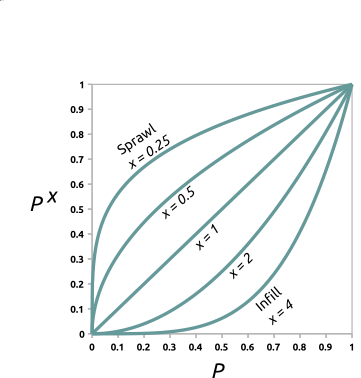

Figure: Transforming development potential surface using incentive tables with different power functions.

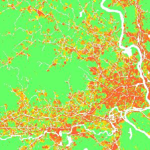
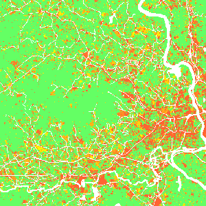
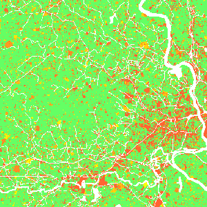
Figure: Effect of incentive table on development probability: infill (left), status quo (middle), sprawl (right) scenario.

Additionally, parameter potential_weight (raster map from -1 to 1) enables users to include policies (such as new regulations or fees) which limit or encourage development in certain areas. Where potential_weight values are lower than 0, the probability surface is simply multiplied by the values, which results in decreased site suitability. Similarly, values greater than 0 result in increased site suitability. The probability surface is transformed from initial probability p with value w to p + w - p * w.

Parameters zoning (raster containing zoning district IDs) and zoning_effects (table containing zoning effects corresponding to zoning district IDs) enable users to include land use regulations (e.g., zoning) which constrain or incentivize development. zoning can be used alone or in combination with zoning_effects. If zoning_effects is not provided, any or all of the following zoning IDs should be present in the zoning raster and the predefined zoning effects are applied.

Zoning District Zoning ID Zoning Effect

High-Density Residential 100 0

Medium-High Density Residential 101 -0.124

Medium Density Residential 110 -0.440

Medium-Low Density Residential 120 -0.656

Low-Density Residential 130 -0.780

Rural Residential 131 -0.790

Commercial 200 -0.157

Industrial 201 -0.026

Office 202 -0.127

Parks and Recreation 203 -0.817

Mixed Use 300 -0.105

Planned Use 301 0.115

Downtown 302 -1

No Zoning 0 0

Where zoning effects are lower than 0, site suitability is decreased, when greater than 0 site suitability is increased. For zoning effect (w') less than 0, site suitability (p) is adjusted following p(1 - |w'|). If zoning effects are greater than 0, site suitability is adjusted following p + w' - p * w'. Note: If part of your study region does not have zoning, or you do not wish to apply the zoning effect to part of your study region, you may assign zoning ID 0 to those areas.

Users can also optionally provide unique zoning effects (values between -1 and 1) or regional stringency values (values between 0 and 2) in zoning_effects table. Stringency values adjust the magnitude of the effect of each zoning district by region. Values less than 1 reduce the magnitude of zoning effects while values greater than 1 increase the magnitude. Given zoning effect w and stringency s, adjusted zoning effects w' = max(-1, min(1, w * s)).

Examples of zoning_effects table
Region_ID values in the first column should align with region IDs in subregions raster and zoning ID column headers should align with zoning IDs in zoning raster.

Providing unique zoning IDs (1, 2) and effects, but no regional stringency (set to 1):

Zoning District	Zoning ID	Zoning Effect
High-Density Residential	100	0
Medium-High Density Residential	101	-0.124
Medium Density Residential	110	-0.440
Medium-Low Density Residential	120	-0.656
Low-Density Residential	130	-0.780
Rural Residential	131	-0.790
Commercial	200	-0.157
Industrial	201	-0.026
Office	202	-0.127
Parks and Recreation	203	-0.817
Mixed Use	300	-0.105
Planned Use	301	0.115
Downtown	302	-1
No Zoning	0	0

Region_ID,stringency,1,2
1,1,-0.5,0.5
2,1,-0.8,0.3

Using default zoning IDs and effects, but providing regional stringency values:

Region_ID,stringency
1,0.5
2,1.5

Output

After the simulation ends, raster specified in parameter output is written. If optional parameter output_series is specified, additional output is a series of raster maps for each step. Cells with value 0 represents the initial development, values >= 1 then represent the step in which the cell was developed. Undeveloped cells have value -1.

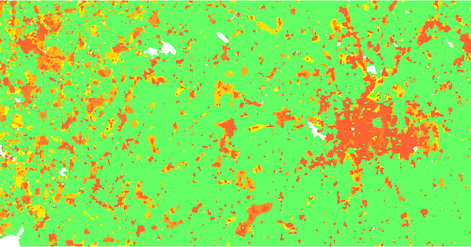
Figure: Output map of developed areas

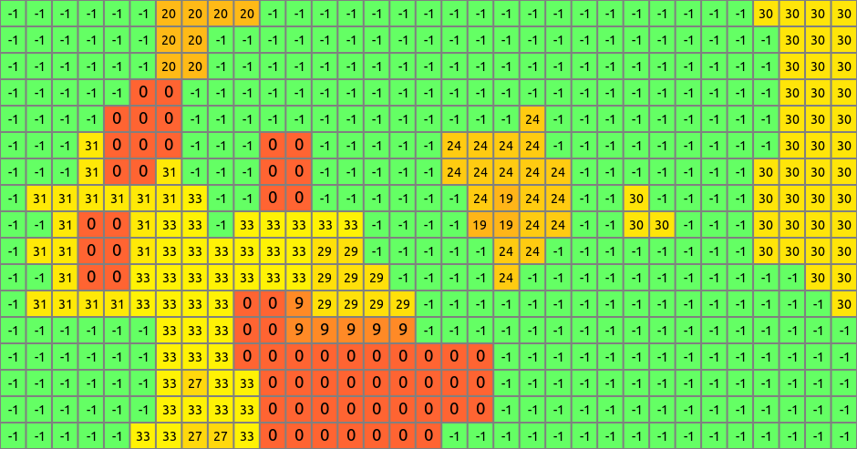
Figure: Detail of output map

Climate forcing

Climate forcing submodel estimates the probability that a developed pixel will experience flood damage and the likely adaptation response (protect and armour, retreat, or stay trapped). Response is based on flood probability, level of damage, and local estimates of adaptive capacity. Climate forcing submodel integrates current and future flood probability and flood depth data with the adaptive capacity of developed pixels to probabilistically predict flood severity and the response evoked by flooding in a developed pixel. The model also predicts the within- or between-county destinations of displaced residents.

The input flood_maps_file includes flood depth data for different flood probabilities for different steps of the simulation:

step,probability,raster
1,0.05,flood_20yr_2020_depth
1,0.01,flood_100yr_2020_depth
1,0.002,flood_500yr_2020_depth
11,0.05,flood_20yr_2030_depth
11,0.01,flood_100yr_2030_depth
11,0.002,flood_500yr_2030_depth

Alternatively, if such detailed data are not available, one can use floodplain raster of given flood return period together with HAND (Height Above Nearest Drainage) raster (hand option) derived from a DEM to estimate flood depth automatically (experimental). Flood probablity raster then contains the probability values (e.g., 0.01 for a 100-yr flood).

step,raster
1,flood_probability_2020
11,flood_probability_2030

Option hand_percentile influences the derived depth, high values (> 90) tend to overestimate the flood depth.

Flood events are stochastically simulated on the level of HUCs (e.g., HUC 12), use huc input option for raster representation of HUCs. Use flood_logfile to log the simulated flood events into a CSV file for further information (step, HUC ID, flood probability).

Once a flood event is simulated, local damage is estimated using flood-damage curves provided in a CSV file in option depth_damage_functions. Its header includes inundation levels in vertical units. The first column is an id of a subregion given in ddf_subregions and the values are percentages of structural damage.

ID,0.3,0.6,0.9
101,0,15,20
102,10,20,30

Once the damage is established, response is stochastically evaluated based on the adaptive_capacity raster with values ranging from -1 (most vulnerable) to 1 (most resilient). Option response_func evaluates the response based on the damage and adaptive capacity, e.g., with high damage vulnerable populations are less likely to protect and armour (adapt) than higly resilient populations. Responses include 1) retreat resulting in pixel abandonment, 2) stay and adapt, and 3) stay trapped. When a pixel is abandoned, the redistribution_matrix is used to decide to which subregion the pixel is moved. It contains probabilities of moving from one subregion to another:

ID,37013,37014,...
37013,0.6,0.01,...
37014,0.05,0.3,...

Output file redistribution_output can be used to log the redistribution happening during the simulation.

EXAMPLE

r.futures.simulation -s developed=lc96 predictors=d2urbkm,d2intkm,d2rdskm,slope \
  demand=demand.txt devpot_params=devpotParams.csv discount_factor=0.6 \
  compactness_mean=0.4 compactness_range=0.08 num_neighbors=4 seed_search=probability \
  patch_sizes=patch_sizes.txt development_pressure=gdp n_dev_neighbourhood=10 \
  development_pressure_approach=gravity gamma=2 scaling_factor=1 \
  subregions=subregions incentive_power=2 \
  potential_weight=weight_1 output=final_results output_series=development

REFERENCES

Meentemeyer, R. K., Tang, W., Dorning, M. A., Vogler, J. B., Cunniffe, N. J., & Shoemaker, D. A. (2013). FUTURES: Multilevel Simulations of Emerging Urban-Rural Landscape Structure Using a Stochastic Patch-Growing Algorithm. Annals of the Association of American Geographers, 103(4), 785-807. DOI: 10.1080/00045608.2012.707591
Dorning, M. A., Koch, J., Shoemaker, D. A., & Meentemeyer, R. K. (2015). Simulating urbanization scenarios reveals tradeoffs between conservation planning strategies. Landscape and Urban Planning, 136, 28-39. DOI: 10.1016/j.landurbplan.2014.11.011
Petrasova, A., Petras, V., Van Berkel, D., Harmon, B. A., Mitasova, H., & Meentemeyer, R. K. (2016). Open Source Approach to Urban Growth Simulation. Int. Arch. Photogramm. Remote Sens. Spatial Inf. Sci., XLI-B7, 953-959. DOI: 10.5194/isprsarchives-XLI-B7-953-2016
Sanchez, G.M., A. Petrasova, A., M.M. Skrip, E.L. Collins, M.A. Lawrimore, J.B. Vogler, A. Terando, J. Vukomanovic, H. Mitasova, and R.K. Meentemeyer (2023). Spatially interactive modeling of land change identifies location-specific adaptations most likely to lower future flood risk. Sci Rep 13, 18869. DOI: 10.1038/s41598-023-46195-9

AUTHORS

Corresponding author:
Anna Petrasova, akratoc ncsu edu, Center for Geospatial Analytics, NCSU

Original standalone version:
Ross K. Meentemeyer,
Wenwu Tang,
Monica A. Dorning,
John B. Vogler,
Nik J. Cunniffe,
Douglas A. Shoemaker
(Department of Geography and Earth Sciences, UNC Charlotte)
Jennifer A. Koch (Center for Geospatial Analytics, NCSU)

Port to GRASS and GRASS-specific additions:
Vaclav Petras, NCSU GeoForAll

Development pressure, demand, calibration, validation, preprocessing tools and maintenance:
Anna Petrasova, NCSU GeoForAll

Climate forcing submodel:
Anna Petrasova, NCSU GeoForAll
Georgina Sanchez, Center for Geospatial Analytics, NCSU

Zoning:
Margaret Lawrimore, Center for Geospatial Analytics, NCSU
Anna Petrasova, NCSU GeoForAll

SOURCE CODE

Available at: r.futures.simulation source code (history)

Accessed: Monday Jul 27 12:29:20 2026